
How long will you wait?
Math Puzzle #6

Problem
You work in a very large bus service company and you have been tasked with checking the punctuality of the town’s bus service. The company claims that they schedule around 4 buses per hour, i.e. about 1 bus every 15 minutes on average (not exactly uniformly, but they try to maintain that 4 buses are released from the depot in an hour).
To inspect this claim, you decide to drop at a random time every day, and ask the people waiting at the bus stop about how long they’ve been waiting, and also wait till the next bus arrives. You keep doing this for a week, and find that the average waiting time was around 15 mins! If you think intuitively, you should have had observed that the average waiting time for you would be half of 15 mins, i.e. 7.5 minutes. Bummer!
Now unless you are in Japan, you would have observed this yourself. If you arrive at a station, where they claim that there would be a bus/train around every 15 minutes; then more often than not, you would have waited for 15 minutes, or maybe even more! Are you just unlucky? Or is this some statistical paradox?

Solution
Let’s clear out some ambiguity in the question, which often comes up when people first hear this. If the buses arrive exactly every ten minutes, it’s true that your average wait time will be half that interval: five minutes. In real-life and this question too, the buses often wait come from different routes, have different speeds, and are not able to maintain the exact time schedule. We are currently focusing on a bus vs time distribution where the average time gap is known. This distribution is known as the Poisson distribution (people with a background in probability distributions would be familiar with it, if not try this - 1, 2). The key to understanding the question is that the two-time intervals reported earlier are actually measuring different things!
If the time interval only focused on is 60 mins, and the instances at which the buses arrived are (a, b, c, d), where they belong to [0,60]. Now, since they are sampled from a distribution where the average of the time gaps is: 15 minutes. Thus, the values can be (5 min, 15 min, 55 min, 60 min). You can see that the average of the time gaps is 15 minutes. This is an exaggerated example to help you understand, but this would help!
Now when you randomly arrive at this hour, you can choose any of the gaps, but this would not be uniform. Since the length of the time intervals is different. Most likely you’ll arrive in the time interval between 15 mins and 55 mins! Then you would be waiting much more than 7.5 minutes.
E(waiting time) = (1/2)[(5/60)*(5) + (10/60)*(10) + (40/60)*40 + (5/60)*5]=14.58 minutes
The additional 1/2 comes from the fact that if we arrive in a time interval of let’s say 30 minutes, then the time we wait would be around 15 minutes if we assume we arrive completely randomly within that time. In notation, the expectation of the arrival times is:
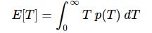
where p(T) is the distribution of intervals T between buses as they arrive at the bus stop. The expected wait time E[W] would then be half of the expected interval experienced by passengers so, E[W] = 0.5*E[T].
If the buses are exactly accurate then the time you wait is around half the expected time interval between arrivals, but if the schedules are not exact, you would end up waiting more time!
This paradox is known as the inspection paradox and is something very interesting to read. It shows how often our intuition fails while modeling the process itself, and we statistics is often a science where half-knowledge is worse than nothing.
Some math theory!
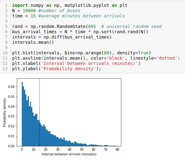
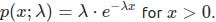
We cheat around in order to get a more concrete mathematical answer. If we assume that the time instances are randomly sampled and the number of buses is quite large, we can check the histogram of the time intervals, we will see that it follows an exponential distribution. The exponential distribution of intervals implies that the arrival times follow a Poisson process (thread - 3). This allows us to write some math, and get an answer too!
If we denote the waiting time as a random variable X following the exponential distribution (the value of lambda would be corresponding to an inverse of average waiting time, according to the above argument)
Then the expected value for this distribution is E(X) = 1/λ, which can be interpreted as your waiting time. Interestingly, this gives us another perspective that it doesn’t matter when you arrive to the bus stand, the probability of the event that you have to wait t more minutes is the same as the probability of the event that you have wait t more minutes, given you have come any time before!
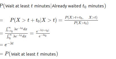
The Poisson process is a memory-less process that assumes the probability of arrival is entirely independent of the time since the previous arrival. In reality, however, if someone decides to create a bus-schedule, he will try to deliberately avoid this, and rather begin their routes on a schedule that best serve the transit-riding public.
If you like this newsletter, please drop a like and share it with your friends! You can reach us if you have any suggestions and we’ll be happy to take note.